物理与统计,从零开始Physics and statistics, from zero
假设你只学过微积分和基础概率。本页把项目用到的每个概念按顺序讲一遍,每个概念配一个算例和一张图。
Suppose you only know calculus and basic probability. This page builds up every concept the project uses, in order, each with one worked number example and one figure.
- 泊松计数与光变曲线Poisson counts and light curves
- GTI 与保留比例 f_TGTI and the retained fraction f_T
- 活时间:EXPOSU、TIMEDEL、FRACEXPLive time: EXPOSU, TIMEDEL, FRACEXP
- Cash 统计量与对数抛物线连续谱The Cash statistic and the log-parabola continuum
- 连续谱比值 R = C_all/C_KThe continuum ratio R = C_all/C_K
- 线门 L_K/L_B 与能段不相交The line gate L_K/L_B and disjoint bands
- 耦合 s 与故障注入The coupling s and fault injection
- 循环移位零假设、z_null、配对差 z_ΔThe shift null, z_null, and the paired z_delta
- FWER、符号检验、Stouffer ZFWER, the sign test, Stouffer Z
- 预注册、盲测、代码冻结Pre-registration, blinding, code freeze
- 未曝光角落作为粒子监测器The unexposed corner as a particle monitor
1. 泊松计数与光变曲线1. Poisson counts and light curves
X 射线探测器数的是光子个数。单位时间内到达的光子数服从泊松分布 (Poisson distribution):P(n) = μne−μ/n!,均值 μ = rate × time。算例:某 FOV 的 2.5–8 keV 计数率是 2.0 count/s,一个 100 s 的 cell 平均有 μ = 200 个光子;泊松涨落的标准差是 √μ ≈ 14.1,即相对涨落约 7%。光变曲线 (light curve)就是把每个 cell 的计数率画成时间序列。耀斑就是一串显著高于基线的 cell。
An X-ray detector counts photons. The number arriving per unit time follows the Poisson distribution: P(n) = μne−μ/n!, with mean μ = rate × time. Worked example: a FOV 2.5-8 keV rate of 2.0 count/s gives μ = 200 photons in a 100 s cell; the Poisson fluctuation is √μ ≈ 14.1, a relative spread of about 7%. A light curve plots the per-cell rate against time. A flare is a run of cells significantly above the baseline.
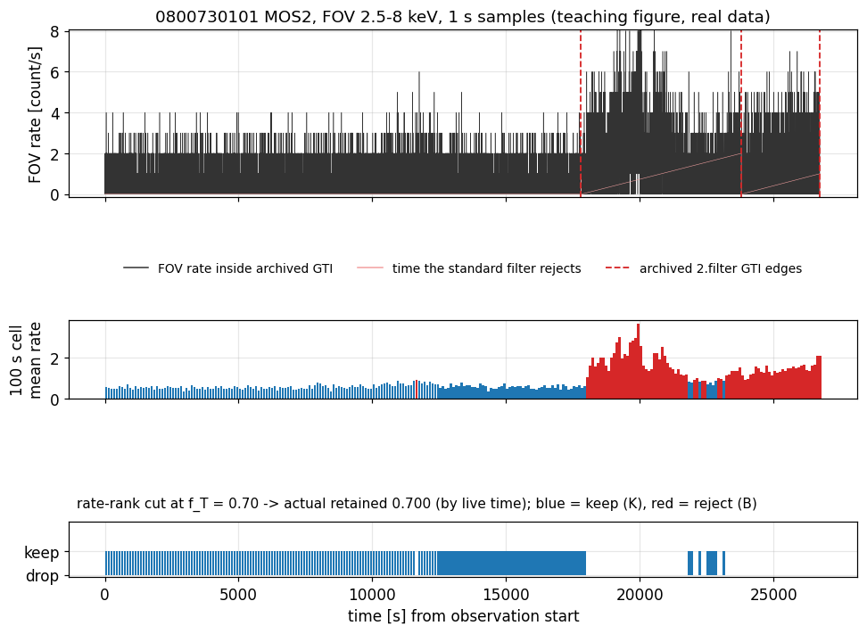
/u/Lang3/program/CDFS/inputs/m31_sirius_temporal_20260902/0800730101/rpc/2.filter/mos2S002-fovlc.fits (只读,astropy 读取)(read-only, read with astropy)
2. GTI 与保留比例 f_T2. GTI and the retained fraction f_T
好时间段 (good time interval, GTI)是一张"哪些时间能用"的清单:FITS 文件里就是一列 (START, STOP) 区间。筛掉耀斑 = 把坏时间写成 GTI 的补集(BTI)。保留比例 f_T = T_K/T_all,其中 T_K 是保留的活时间(不是墙钟时间!)。算例:0800730101 MOS2 的归档 2.filter 保留 f_T = 0.6922,即 26,371 s 里留 18,254 s。注意不同观测的 f_T 差别很大:0800730401 几乎不删 (f_T = 0.9988),0800731801 删掉 70% (f_T = 0.2949)。
A good time interval (GTI) is a list of "which times are usable": in a FITS file, a column of (START, STOP) intervals. Flare screening = writing the bad time as the complement of the GTI (the BTI). The retained fraction is f_T = T_K/T_all, where T_K is the retained live time (not wall-clock time!). Worked example: the archived 2.filter of 0800730101 MOS2 keeps f_T = 0.6922 — 18,254 s out of 26,371 s. Retention varies hugely across observations: 0800730401 keeps almost everything (f_T = 0.9988), 0800731801 cuts 70% (f_T = 0.2949).
legacy/results/.../line_continuum_invariant.json (每 ObsID 的 archived_2filter f_T)(per-obsid archived_2filter f_T)3. 活时间:EXPOSU、TIMEDEL、FRACEXP3. Live time: EXPOSU, TIMEDEL, FRACEXP
CCD 读书时不能同时曝光,所以每个时间 bin 有一个"活着的比例" FRACEXP,bin 长 TIMEDEL。一个 cell 的活时间 = Σ TIMEDEL × FRACEXP。为什么不能用"有事件就记满 100 s"?因为 0.9% 的 cell 活时间坍缩(低活时间),它们的"率"被高估到中位数 4.87 倍,恰好被率排名推到耀斑一侧 —— 实测在 0.70 保留率下,5395 个 cell 里有 79 个因此站错了边,比真正的坏 cell(49 个)还多。规则:做归一化无所谓,做判别量绝不行。GTI 构造是后者。
A CCD cannot expose while it reads out, so every time bin has a "live fraction" FRACEXP over a bin length TIMEDEL. A cell's live time = Σ TIMEDEL × FRACEXP. Why not just charge 100 s to any cell containing events? Because 0.9% of cells have collapsed live time; their "rate" is overstated by a median factor 4.87 and rate-ranking pushes them exactly to the flare side — measured at retention 0.70, 79 of 5395 cells land on the wrong side of the cut this way, more than the 49 genuinely bad cells. Rule: fine as a normalisation, unusable as a discriminant. GTI construction is the latter.
legacy/cognition-os/insights/I004_constrained_pareto_single_observation_gti.md §活时间§Live exposure4. Cash 统计量与对数抛物线连续谱4. The Cash statistic and the log-parabola continuum
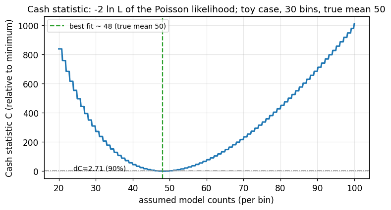
计数很少时,χ² 不适用;要用泊松似然。W. Cash (1979) 定义 C = −2 ln L,对泊松数据(忽略常数项)每 bin 贡献 2(m − n + n ln(n/m)),m 是模型,n 是数据。算例:30 个 bin、真均值 50,模型取 m = 50 时 C 最小;取 m = 40 时 ΔC = 2×30×(40−50+50 ln(50/40)) ≈ 2×30×(−10+11.78) ≈ 107。ΔC = 1 对应单参数 1σ,ΔC = 2.71 对应 90%。对数抛物线 (log-parabola)是连续谱模型:A(E) = K·(E/E₀)−γ−β·ln(E/E₀),比纯幂律多一个曲率项 β。为什么不用幂律?因为在 1.0–2.4 keV 窗口内,静态谱的似然比检验拒绝裸幂律(ΔC 中位数 9.1,17/23 观测超过 99% 置信)。
With few counts χ² does not apply; use the Poisson likelihood. W. Cash (1979) defined C = −2 ln L; for Poisson data (dropping constants) each bin contributes 2(m − n + n ln(n/m)), with m the model and n the data. Worked example: 30 bins, true mean 50; the minimum is at m = 50; at m = 40, ΔC = 2×30×(40−50+50 ln(50/40)) ≈ 2×30×(−10+11.78) ≈ 107. ΔC = 1 is 1σ for one parameter; ΔC = 2.71 is 90%. The log-parabola is the continuum model: A(E) = K·(E/E₀)−γ−β·ln(E/E₀) — a power law plus a curvature term β. Why not a bare power law? Because within the 1.0-2.4 keV window the quiescent spectrum rejects it by likelihood ratio (ΔC median 9.1; 17/23 observations above 99% confidence).
legacy I004
legacy I004
5. 连续谱比值 R = C_all/C_K5. The continuum ratio R = C_all/C_K
对每次观测,先对全部时间的光谱做一次 Cash 拟合,得连续谱计数率 C_all;再对候选 K 的光谱拟合,得 C_K。定义 R = C_all/C_K。R > 1 说明保留时间的连续谱比全时段低 —— 删掉的时间确实更亮。算例(0800730101 MOS2,归档 2.filter):C_all = 0.5911 count/s,C_K = 0.3779 count/s,R = 1.564。为什么 R 不能跨观测合并?因为它的上限由该观测自己的耀斑含量决定:同一候选(归档 2.filter)在 30 次观测里的 R 从 1.0(没耀斑)到 11.8(大耀斑)。平均或排名 R 就是把不同物理条件混在一起。
For each observation, fit the Cash model to the all-time spectrum to get the continuum rate C_all, and to the candidate-K spectrum to get C_K. Define R = C_all/C_K. R > 1 means the retained time has a lower continuum than the observation as a whole — the discarded time really was brighter. Worked example (0800730101 MOS2, archived 2.filter): C_all = 0.5911 count/s, C_K = 0.3779 count/s, R = 1.564. Why can R not be pooled across observations? Its ceiling is set by each observation's own flare content: the same candidate (archived 2.filter) spans R from 1.0 (no flares) to 11.8 (big flares) over the 30 observations. Averaging or ranking R mixes different physical conditions.
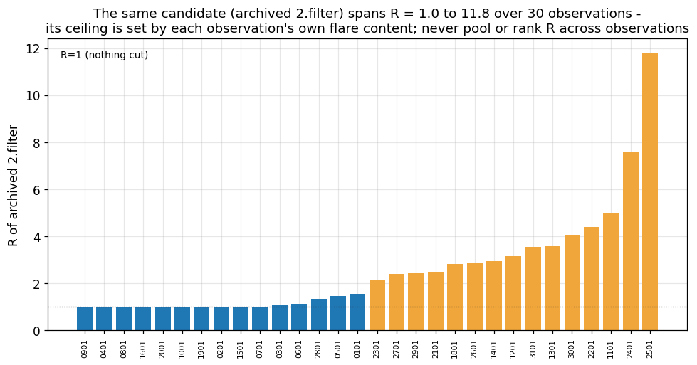
legacy/results/m31_mos2_line_continuum_invariant_20260910_g1/line_continuum_invariant.json (30 个 case 的 archived_2filter R)(archived_2filter R for the 30 cases)
6. 线门 L_K/L_B 与能段不相交6. The line gate L_K/L_B and disjoint bands
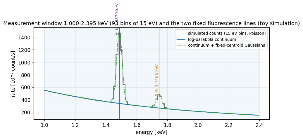
R 有一个漏洞:如果选择能段与测量窗口重叠,那么"挑连续谱低的 cell"会同时压低线率,门就会自证通过。实测在禁止的重叠配置下,干净观测上 L_K/L_B 掉到 0.768/0.803(z = −5.4/−4.6),R 却虚高到 1.074/1.085(+5.5/+6.1σ)—— 什么都没有的观测被制造出 6σ 的"发现"。它恰好污染最干净、被用作零控制的观测。所以三条能段必须互不相交:2.5–8.0 keV 选择、1.000–2.395 keV 测量、<1 keV 是科学段。线门本身比较 K 与其不相交补集 B 的 Al-K 线率:L_K/L_B 应与 1 相容;若保留时间的线率显著低,说明选择把线也删了,门报警。线中心固定(Al-K 1.4879、Si-K 1.7466 keV),因为观测间 E_Al 散布只有 0.9 eV,而"保留 vs 弃掉"之间移动 −0.04 ± 0.44 eV。
R has a hole: if the selection band overlaps the measurement window, "picking low-continuum cells" also depresses the line rate, and the gate passes itself. Measured in the forbidden overlapping configuration, on clean observations L_K/L_B falls to 0.768/0.803 (z = −5.4/−4.6) while R is inflated to 1.074/1.085 (+5.5/+6.1σ) — a 6σ "discovery" manufactured from an observation with nothing to find. It corrupts exactly the cleanest observations used as zero controls. Hence the three bands must be disjoint: 2.5-8.0 keV selects, 1.000-2.395 keV measures, and below 1 keV is the science band. The gate itself compares the Al-K rate in K with its disjoint complement B: L_K/L_B should be compatible with 1; if the retained-time line rate is significantly low, the selection deleted the line too and the gate fires. The line centroids are fixed (Al-K 1.4879, Si-K 1.7466 keV) because E_Al scatters only 0.9 eV between observations and moves −0.04 ± 0.44 eV between kept and rejected time.
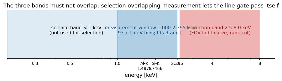
legacy I004; g1 line_continuum_invariant.json overlap_diagnostic
动画:K vs B 光谱与线比Animation: K vs B spectra and the line ratio
toy 模拟:K 是安静时间,B 的连续谱更高(模拟软质子)但线率相同。若删的只是线无关的连续谱,ln(L_K/L_B) 应接近 0.0。
Toy simulation: K is quiet time; B has a higher continuum (simulating soft protons) but the same line rate. If only line-free continuum was removed, ln(L_K/L_B) should be near 0.0.
7. 耦合 s 与故障注入7. The coupling s and fault injection
拟合里线与连续谱不独立:往干净光谱里注入纯连续谱(真线率按构造不变),拟合出的线率会漂移。这就是耦合,记作 s = d lnL/d lnC。注入实验(60 个泊松实现 × 3 个注入水平)测得 s = −0.0128 ± 0.0039(−3.3σ):注入更多连续谱,拟合线率反而降低。注意历史教训:2026-09-14 之前,一次基于观测间回归的估计给出 +0.0098 ± 0.0063(1.6σ),并据此提出过修正 —— 后来被注入实验推翻(符号相反),修正被撤回。s 的修正至今未应用:门内值与"反事实修正后"值都报告,但只用门内值做门判决。
In the fit, the line and the continuum are not independent: inject pure continuum into a clean spectrum (the true line rate unchanged by construction) and the fitted line rate drifts. This is the coupling, s = d lnL/d lnC. The injection experiment (60 Poisson realisations × 3 injection levels) gives s = −0.0128 ± 0.0039 (−3.3σ): more injected continuum, lower fitted line rate. A historical lesson: before 2026-09-14, an observational regression estimated +0.0098 ± 0.0063 (1.6σ) and a correction was proposed on that basis — later overturned by the injection experiment (opposite sign), and the proposal withdrawn. The s correction remains unapplied: both the as-gated and the "counterfactual-corrected" values are reported, but only the as-gated value decides the gate.
g1 fault_injection.json coupling_calibration; legacy I004 §开放项§open items8. 循环移位零假设、z_null、配对差 z_Δ8. The shift null, z_null, and the paired z_delta
R 的显著性不能用解析传播,因为 K 嵌套在全时间里、选择依赖数据。项目用循环移位零假设 (circular-shift null):把"保留掩码"在活时间坐标里随机平移一段,重新拟合,重复 200 次,得到 R 的零分布;z_null = (R − mean)/sd。算例(0800730101,归档 2.filter):R = 1.564,零分布 mean = 0.9978、sd = 0.0257 → z_null = 22.1,即这次筛选删的时间显著高于随机。配对差用于 E3:两个掩码(2.filter 与匹配率排名)按同一个随机移位滚动,Δ = ln R(b) − ln R(a) 的零分布给出 z_Δ。用同一个移位是为了让两个高度相关的统计量的差有正确的宽度。
The significance of R cannot use analytic propagation, because K is nested in all-time and the selection is data-dependent. The project uses a circular-shift null: randomly roll the "keep mask" along the live-time coordinate, refit, repeat 200 times, and read the null distribution of R; z_null = (R − mean)/sd. Worked example (0800730101, archived 2.filter): R = 1.564, null mean = 0.9978, sd = 0.0257 → z_null = 22.1 — the discarded time is significantly brighter than random. The paired difference is used in E3: both masks (2.filter and matched rate-rank) are rolled by the same random shift, and the null of Δ = ln R(b) − ln R(a) gives z_Δ. The same shift keeps the width of the difference of two highly correlated statistics correct.
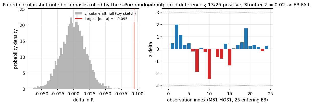
results/p001_m31_mos1/p001_endpoints_m31.json (E3 rows)
动画:循环移位零假设Animation: the circular-shift null
点"抽一次"做 10 次随机移位;直方图积累起来就是 Δ 的零分布。红线是观测到的 Δ。
Click "one draw" for 10 random shifts; the accumulating histogram is the null of Δ. The red line is the observed Δ.
9. FWER、符号检验、Stouffer Z9. FWER, the sign test, Stouffer Z
族错误率 (family-wise error rate, FWER):做了 N 次检验,至少一次假阳性的概率。E1 要求零控制观测上、全体候选的 |z_null| ≥ 3 比例 ≤ 0.05 —— 不是单点,是全家。算例:MOS1 有 9 个零控制观测 × 78 个候选,0 个假阳性 → FWER 通过。符号检验 (sign test):25 次观测的 Δ,若真实效果为 0.0,正负各半;13 正的单侧 p = 0.50 —— 与掷硬币无异。Stouffer Z:把每次观测的 z_Δ 直接平均再乘 √n:Z = Σz/√n = 0.02 —— 25 个约 ±1 的 z 平均后应约 1/√n,实测 0.02 说明没有任何共同方向的信号。
The family-wise error rate (FWER): with N tests, the probability of at least one false positive. E1 requires the fraction of candidates with |z_null| ≥ 3 on the zero-control observations to be ≤ 0.05 — over the whole family, not a single point. Worked example: MOS1 has 9 zero-control observations × 78 candidates, 0 false positives → FWER passes. The sign test: 25 observation Δs; if the true effect is 0.0, half are positive; 13 positive gives a one-sided p = 0.50 — indistinguishable from a coin flip. The Stouffer Z: average the per-observation z_Δ and multiply by √n: Z = Σz/√n = 0.02 — 25 z's of about ±1 should average to about 1/√n; the measured 0.02 means there is no signal in any common direction.
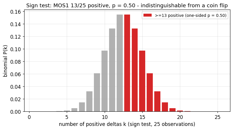
results/p001_m31_mos1/p001_endpoints_m31.json (E3: n_positive = 13, sign p = 0.5)
动画:25 个 Δ → 合并判决Animation: 25 deltas → one verdict
真实 MOS1 E3 数字。正的个数给符号检验 p;z 的平均给 Stouffer Z;两者都不达阈值 → E3 FAIL。
Real MOS1 E3 numbers. The count of positives gives the sign-test p; the mean of the z's gives the Stouffer Z; neither meets the thresholds → E3 FAIL.
10. 预注册、盲测、代码冻结10. Pre-registration, blinding, code freeze
预注册 (pre-registration):在看到数据结果之前,把问题、方法、统计量、阈值、集合全部写死。项目只认这种证据,因为历史教训:r16 规则在单观测前沿上"看起来很好",迁移到 30 个观测后 10/8(p = 0.50)—— 单观测前沿挖掘选出的是噪声。盲测 (blinding):盲集的数据不被任何探索代码触碰;改代码先在已消费的 M31 MOS2 上测试并复现 g1 收据。代码冻结 (code freeze):P001 批准后,代码连同 git 哈希(46d8df3)一起冻结;任何修改都是新的预注册(P002…),修正案必须带日期、在看到结果前批准。E3 失败了也要如实报告 —— 这正是预注册的意义:负结果同样有证据价值。
Pre-registration: write down the question, method, statistic, thresholds and sets before seeing any outcome. The project accepts only this kind of evidence, because of the historical lesson: the r16 rule "looked good" on the single-observation frontier, yet transferred to 30 observations at 10/8 (p = 0.50) — single-observation frontier mining selects noise. Blinding: blind-set data is never touched by exploratory code; code changes are tested on consumed M31 MOS2 and reproduce the g1 receipt first. Code freeze: once P001 was approved the code was frozen with its git hash (46d8df3); any change is a new pre-registration (P002…), and amendments must be dated and approved before outcomes are seen. An E3 failure is reported as such — that is the point of pre-registration: negative results carry evidentiary value too.
11. 未曝光角落作为粒子监测器11. The unexposed corner as a particle monitor
MOS 相机的视场 (FOV) 是圆形;圆形之外、探测器边缘之内有几个角落,望远镜的光永远照不到。这些未曝光角落 (unexposed corner)只接收粒子(宇宙线打到相机结构上的次级辐射),不接收聚焦的软质子或天体光子。因此角落的 2.5–8 keV 计数率 Q 是一个"纯粒子监测器":若保留时间 K 与弃掉时间 B 的粒子水平不同,ln(Q_K/Q_B) 应偏离 0。算例(0800730101 MOS1,归档 2.filter 的 K/B 切分):N_K = 1391、T_K = 15,700 s → Q_K = 0.0886 count/s;N_B = 961、T_B = 11,052 s → Q_B = 0.0870 count/s;ln(Q_K/Q_B) = 0.019 ± 0.042 —— 单次观测精度约 4%,太粗。P001 把 29 次观测逆方差加权叠加:MOS1 σ = 0.0133(> 0.010,太吵),MOS2 σ = 0.0098(勉强可用)。两台相机都看不到 ~1% 的差异。
The MOS field of view (FOV) is circular; outside the circle but inside the detector are corners that telescope light never reaches. These unexposed corners receive only particles (secondaries from cosmic rays striking the camera structure), never focused soft protons or celestial photons. The corner 2.5-8 keV rate Q is therefore a "pure particle monitor": if the particle level differs between kept time K and rejected time B, ln(Q_K/Q_B) should deviate from 0. Worked example (0800730101 MOS1, K/B split of the archived 2.filter): N_K = 1391 over T_K = 15,700 s → Q_K = 0.0886 count/s; N_B = 961 over T_B = 11,052 s → Q_B = 0.0870 count/s; ln(Q_K/Q_B) = 0.019 ± 0.042 — a single observation has ~4% precision, too coarse. P001 stacks 29 observations with inverse-variance weighting: MOS1 σ = 0.0133 (> 0.010, too noisy), MOS2 σ = 0.0098 (usable by a hair). Neither camera sees a ~1% difference.
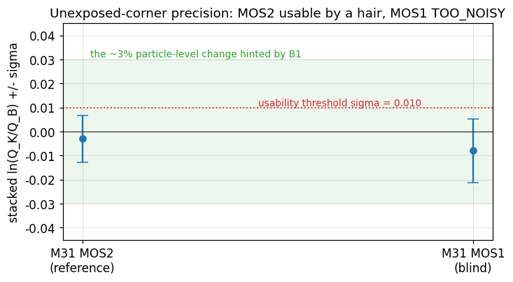
results/p001_m31_mos1/p001_endpoints_m31.json (E5 corner blocks)